Load a real professional match, the ISL 2021/22 final, in a few lines of Python. Count events, compare shots and xG, find the busiest passers and draw a shot map. Free data, tested code, and the two data traps that catch beginners.
You can start football analytics with Python today, for free, using real professional match data. This tutorial takes one real match, the 2021/22 Indian Super League final between Hyderabad and Kerala Blasters, and in about 40 lines of Python counts every event, compares shots and expected goals (xG), finds the busiest passers and draws a shot map.
You need Python 3 and three libraries: pandas, matplotlib and requests (pip install pandas matplotlib requests). No account, no API key. The data is StatsBomb’s free open data, which includes the full ISL 2021/22 season. Every output below is what the code printed when we ran it.
Step 1: load the season and find the final
StatsBomb publishes one file listing a season’s matches and one file of events per match. The ISL 2021/22 season is competition 1238, season 108.
import requests
import pandas as pd

BASE = "https://raw.githubusercontent.com/statsbomb/open-data/master/data"

# Every match in the Indian Super League 2021/22 (competition 1238, season 108)
matches = pd.DataFrame(requests.get(f"{BASE}/matches/1238/108.json").json())
print(len(matches), "matches")

# Find the final
stage = matches["competition_stage"].apply(lambda c: c["name"])
final = matches[stage == "Championship - Final"].iloc[0]
print(final["match_date"], final["match_id"])115 matches
2022-03-20 3827767A real-world lesson straight away: in this season file, the final’s home team appears as “SC Delhi”. The event file names the same team ID (7289) “Hyderabad”, and the match was Hyderabad against Kerala Blasters. Data has errors. Check a result you already know before trusting a whole dataset, and match teams by ID, not name.
Step 2: load every event in the match
An event is anything that happens on the ball: a pass, a carry, a pressure, a shot. Each one has a type, a team, a player, a minute and a pitch location. pandas’ json_normalize flattens the nested JSON into columns such as type_name and shot_statsbomb_xg.
events = pd.json_normalize(
    requests.get(f"{BASE}/events/{final['match_id']}.json").json(), sep="_"
)
print(len(events), "events")
print(events["type_name"].value_counts().head(6))4096 events
type_name
Pass 1139
Ball Receipt* 996
Carry 873
Pressure 364
Ball Recovery 159
Duel 101
Name: count, dtype: int64Over four thousand events in one match. This is why clubs hire analysts: no one can watch for all of that, but a few lines of code can count it.
Step 3: shots and expected goals
Expected goals (xG) gives every shot a probability of being scored, based on where and how it was taken. Add a team’s xG together and you get the number of goals its chances were worth, which says more about a performance than the score alone.
# Period 5 is the penalty shootout: leave it out of open-play analysis
shots = events[(events["type_name"] == "Shot") & (events["period"] < 5)]

summary = shots.groupby("team_name").agg(
    shots=("id", "count"),
    on_target=("shot_outcome_name",
               lambda s: s.isin(["Goal", "Saved", "Saved To Post"]).sum()),
    xg=("shot_statsbomb_xg", "sum"),
).round(2)
print(summary) shots on_target xg
team_name
Hyderabad 14 6 0.87
Kerala Blasters 16 4 1.19The final finished 1–1 (Rahul K.P. 67′, Sahil Tavora 87′) and Hyderabad won the shootout 3–1. On xG, Kerala Blasters created slightly better chances: 1.19 against 0.87.
Note the period filter. The shootout is stored as period 5, and its penalties carry high xG. Leave it in and the totals jump to 4.00 and 4.32, which is nonsense as a measure of open play. Most beginner mistakes in football data are like this: the code runs, and the number is wrong.
Step 4: who kept the ball moving?
In StatsBomb data a completed pass has no outcome; only incomplete, out or offside passes carry one. So completed passes are the rows where pass_outcome_name is empty.
passes = events[events["type_name"] == "Pass"]
completed = passes[passes["pass_outcome_name"].isna()]   # no outcome = completed
print(completed["player_name"].value_counts().head(5))player_name
Marko Lešković 81
Jeakson Singh Thaunaojam 55
Soraisham Sandeep Singh 52
Lalthathanga Khawlhring 50
Harmanjot Singh Khabra 48
Name: count, dtype: int64All five are Kerala Blasters players, led by centre-back Marko Lešković, well clear of everyone else. Group by team_name instead of player_name and Kerala Blasters completed 461 passes to Hyderabad’s 369. That is a pattern worth a question. Were Kerala Blasters building patiently from the back, or were Hyderabad happy to let their defenders have the ball? Analysis rarely ends with a number; it ends with a better question for the coach.
Step 5: draw a shot map
StatsBomb’s pitch is 120 by 80 units, and event locations are recorded as if each team attacks the same way. So both teams’ shots can go on one half-pitch. Dot size shows xG.
import matplotlib.pyplot as plt
from matplotlib.patches import Rectangle

fig, ax = plt.subplots(figsize=(10, 6.5))
ax.add_patch(Rectangle((0, 0), 120, 80, fill=False))     # pitch, 120 x 80
ax.add_patch(Rectangle((102, 18), 18, 44, fill=False))   # penalty area
ax.add_patch(Rectangle((114, 30), 6, 20, fill=False))    # six-yard box
ax.plot([60, 60], [0, 80], color="black", linewidth=1)   # halfway line

for team, colour in zip(shots["team_name"].unique(), ["tab:blue", "tab:orange"]):
    s = shots[shots["team_name"] == team]
    ax.scatter(s["location"].str[0], s["location"].str[1],
               s=s["shot_statsbomb_xg"] * 900 + 20,
               alpha=0.6, color=colour, label=team)

ax.set_xlim(55, 121); ax.set_ylim(81, -1)
ax.set_aspect("equal"); ax.axis("off"); ax.legend(loc="lower left")
plt.savefig("shot_map.png", dpi=120, bbox_inches="tight")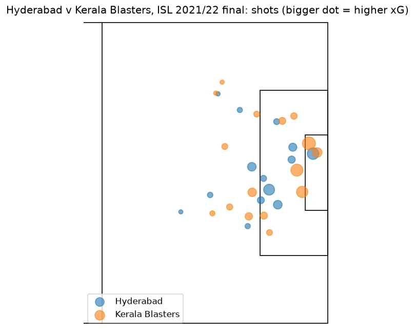
Read it like an analyst. Most of the big dots sit inside the penalty area and close to goal. Kerala Blasters’ largest chances came from close range; many of both teams’ efforts were low-value shots from outside the box.
The skill is not writing the code. It is knowing which number would change a coach’s decision.
Where to go next
- Run the same code on another ISL 2021/22 match: change the filter in Step 1 and everything else works.
- Build a season table of xG for and against for every ISL team, and compare it with the real league table.
- Install mplsoccer, a free library that draws proper pitches, and redo the shot map with it.
- Try passing networks: average player positions, with lines for the most frequent passing combinations.
- Write up one finding in plain English, with a chart. Three projects like that, posted publicly, say more to a club than any certificate.
If you want this taught step by step, our free Football Analytics with Python course on the Sportal learning app covers it with videos, notes and a certificate. It is listed in the sources below. For a full degree in the field, see the B.Sc. in Sports Analytics.
- StatsBomb — Open data — the free event data used throughout; data source: StatsBomb
- StatsBomb — ISL 2021/22 match list — competition 1238, season 108
- StatsBomb — ISL 2021/22 final event file — match 3827767
- Sportal — Football Analytics with Python (free course) — videos, notes and a certificate
- B.Sc. in Sports Analytics — four years, fees published
- Sports analytics skills — what clubs actually look for
- Sports analytics careers in India — roles, pay and routes in
- Free courses — short courses with certificates
Frequently Asked Questions
How do I start football analytics with Python?
Install Python with pandas, matplotlib and requests, then load StatsBomb’s free open data straight from GitHub. One match file gives you every pass, shot and pressure with locations, and in about 40 lines you can compare shots and expected goals and draw a shot map, as this tutorial shows using the ISL 2021/22 final.
Where can I get free football data?
StatsBomb publishes free event data on GitHub for selected competitions, including the full Indian Super League 2021/22 season and several FIFA World Cups. It is free to use for learning and analysis, with StatsBomb credited as the source.
What is xG in football?
Expected goals (xG) is the probability that a shot is scored, based on where and how it was taken. Adding a team’s xG gives the number of goals its chances were worth. In the ISL 2021/22 final, Kerala Blasters created 1.19 xG and Hyderabad 0.87, excluding the penalty shootout.
Do I need to know Python before learning football analytics?
Basic Python helps, but you can learn the two together. This tutorial uses only filtering, counting and one chart. Spreadsheet skills transfer well: pandas is a programmable spreadsheet.
Is there Indian football data for analysis?
Yes. StatsBomb’s open data includes the entire Indian Super League 2021/22 season, 115 matches with full event data, which is free to download.